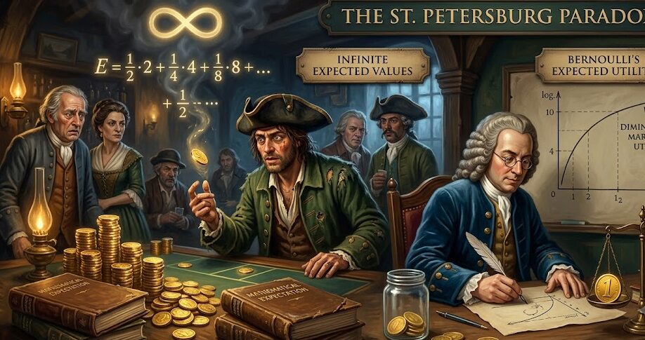
The Infinite Coin-Flip Wager
A fair coin is flipped until it lands on tails. If tails appears on the first flip, the game ends and you receive \$2. If tails appears on the second flip, you receive \$4. In general, if tails appears on the $k$-th flip, you receive $\$2^k$. The mathematical expected value of this game is rigorously infinite ($E(X) = \infty$). Yet, in empirical reality, no rational human being would pay even \$50 to play this game once. Why does classical mathematical expectation fail to capture rational choice?
Presented by Nicolas Bernoulli in 1713 and famously solved by his cousin Daniel Bernoulli in 1738 at the Imperial Academy of Sciences in Saint Petersburg, this paradox represents the historical birth of modern decision theory, microeconomics, and risk-aversion utility modeling.
1. The Classical Divergence: Proving Infinite Expected Value
Let $X$ be the random variable representing the payoff of the game. A fair coin has independent probabilities $P( ext{Heads}) = 1/2$ and $P( ext{Tails}) = 1/2$. The game terminates on the $k$-th toss if and only if the sequence consists of $k-1$ consecutive heads followed by a tail:
P(K = k) = \left( \frac{1}{2} \right)^{k-1} \times \frac{1}{2} = \left( \frac{1}{2} \right)^k = 2^{-k}
The payoff corresponding to outcome $k$ is $x_k = 2^k$. Under the classical definition of mathematical expectation introduced by Christiaan Huygens:
E(X) = \sum_{k=1}^{\infty} P(K = k) \cdot x_k = \sum_{k=1}^{\infty} \left( \frac{1}{2^k} \right) \cdot 2^k = \sum_{k=1}^{\infty} 1 = 1 + 1 + 1 + 1 + \dots = \infty
The infinite series diverges strictly to positive infinity. According to classical decision theory, a rational agent should be willing to pay any finite sum (whether \$1,000, \$1,000,000, or their entire life savings) for a single play of the game. Yet, human participants universally refuse to pay more than \$10 to \$25.
2. Payoff and Probability Distribution Matrix
The table below highlights the extreme tail distribution responsible for the mathematical divergence:
| Flip Count (\(k\)) | Probability (\(P = 2^{-k}\)) | Gross Payoff (\(2^k\)) | Expected Value Contribution (\(P \times 2^k\)) | Cumulative Win Probability |
|---|---|---|---|---|
| 1 | 1/2 (50.0%) | $2 | $1.00 | 50.0% |
| 2 | 1/4 (25.0%) | $4 | $1.00 | 75.0% |
| 3 | 1/8 (12.5%) | $8 | $1.00 | 87.5% |
| 4 | 1/16 (6.25%) | $16 | $1.00 | 93.75% |
| 5 | 1/32 (3.125%) | $32 | $1.00 | 96.875% |
| 10 | 1/1,024 (~0.097%) | $1,024 | $1.00 | 99.902% |
| 20 | 1/1,048,576 | $1,048,576 | $1.00 | 99.9999% |
| 30 | 1/1,073,741,824 | $1,073,741,824 | $1.00 | 99.9999999% |
3. Daniel Bernoulli’s Resolution: Expected Utility Theory
In 1738, Daniel Bernoulli proposed that human beings do not optimize arithmetic wealth $w$, but utility $u(w)$. Bernoulli postulated the principle of diminishing marginal utility: an additional dollar provides less subjective benefit to a wealthy person than to an impoverished person:
du \propto \frac{dw}{w} \implies u(w) = \ln(w)
Let an agent with initial wealth $w_0$ consider paying entrance fee $c$. The expected utility $E[U]$ is:
E[U] = \sum_{k=1}^{\infty} \frac{1}{2^k} \ln(w_0 – c + 2^k)
Because the logarithm grows sub-linearly (concave function: $u”(w) < 0$), this series converges to a finite value! The maximum entrance fee $c^*$ an agent will rationally pay is the Certainty Equivalent, where expected utility equals the utility of status quo: $E[U(w_0 - c^* + X)] = u(w_0)$. For realistic initial wealth ($w_0 = \$1,000$), the fair certainty equivalent collapses to approximately \$10.95.
4. Physical Reality: Finite Bankroll Truncation
Even if an agent possesses linear risk-neutral utility ($u(w) = w$), the paradox fails under physical reality because no casino or counterparty possesses infinite wealth. Let the casino possess a maximum total wealth of $W_{max}$. The game’s payoff is capped at $W_{max}$ once $2^k > W_{max}$.
Suppose the casino is backed by the entire Gross World Product (approximately \$100 trillion $\approx 10^{14} \approx 2^{46.5}$). The maximum number of doubleable tosses is $k = 46$. The truncated expected value is:
E_{finite}(X) = \sum_{k=1}^{46} \frac{2^k}{2^k} + \sum_{k=47}^{\infty} \frac{W_{max}}{2^k} = 46 + W_{max} \cdot 2^{-46} \approx 46 + 1 = \$47.00
Even with the entire economic resources of planet Earth backing the casino, the mathematically fair price to play the game is strictly under \$50!
5. Ergodicity Economics: Time Average vs. Ensemble Average
In recent years, physicist Ole Peters and the London Mathematical Laboratory introduced the concept of ergodicity economics. Classical expected value $E(X) = \infty$ represents an ensemble average: the average outcome across an infinite number of parallel universes playing the game simultaneously.
However, a human being is a non-ergodic system: an individual lives along a single chronological time vector. In time-average growth rate:
g = \lim_{T \to \infty} \frac{1}{T} \ln\left( \frac{W(T)}{W(0)} \right)
If an individual pays a high entrance fee (e.g., \$100) on successive rounds, with 87.5% probability the game pays \$8 or less on each turn. The player’s wealth will hit zero (absorbing state / bankruptcy) with probability 1 long before an astronomical tail event occurs. The St. Petersburg paradox proves that optimizing mathematical ensemble averages in non-ergodic environments leads to inevitable financial ruin.
6. The Multi-Round St. Petersburg Game and Wealth Evolution
While a single round of the St. Petersburg game exhibits an infinite ensemble average, how does a player’s wealth evolve when playing $N$ consecutive rounds? In 1937, mathematician William Feller proved a landmark limit theorem in probability theory regarding the accumulated payoff $S_N = \sum_{i=1}^N X_i$ of $N$ independent St. Petersburg games.
Feller proved that the Weak Law of Large Numbers fails in its standard form because $E(X)$ diverges. Instead, $S_N$ obeys a non-standard scaled limit theorem:
\lim_{N \to \infty} P\left( \left| \frac{S_N}{N \log_2(N)} – 1 \right| < \epsilon \right) = 1
In repeated play, the fair accumulated entrance fee for $N$ games is not linear; it scales as $N \log_2(N)$! If you play $N = 1,000$ rounds, the fair total fee is approximately $1,000 \times \log_2(1,000) \approx 10,000$ dollars (roughly \$10 per round). Only as $N \to \infty$ does the per-round average $\log_2(N)$ diverge toward infinity. A player playing once who pays \$1,000 is effectively paying an upfront premium for an astronomical sample size they will never experience in a human lifetime.
7. Cumulative Prospect Theory and Probability Weighting
In behavioral economics, Daniel Kahneman and Amos Tversky’s Cumulative Prospect Theory (CPT) provides an alternate psychological resolution. CPT demonstrates that humans do not evaluate objective probabilities $p_k$ linearly; they apply a non-linear probability weighting function $w(p)$:
w(p) = \frac{p^\gamma}{(p^\gamma + (1-p)^\gamma)^{1/\gamma}}, \quad \text{with } \gamma \approx 0.65
While humans overweight small probabilities in lottery settings, when probabilities plunge below $10^{-6}$ (such as tossing 20 consecutive heads, $p \approx 10^{-6}$), the human cognitive apparatus treats the probability as virtually zero ($w(p) \to 0$). The mathematical tail that produces the infinite expectation is completely dismissed by the human perceptual system, bounding the subjective value of the game to a modest sum.
9. The Ergodicity Breakdown: Time Averages vs. Ensemble Averages
In contemporary statistical physics and economics, Ole Peters demonstrated that the St. Petersburg Paradox is a primary manifestation of the Ergodicity Problem in Economics. Expected value theory assumes that the system is ergodic—meaning that the average outcome over a large collection of people playing the game once (the ensemble average) is identical to the average outcome of a single individual playing the game repeatedly over time (the time average).
For the St. Petersburg coin toss, while the ensemble average is infinite:
\lim_{M \to \infty} \frac{1}{M} \sum_{j=1}^M X_j = \inftyThe time average growth rate of wealth for a single player reinvesting their capital over $T$ sequential rounds converges with probability 1 to a finite, modest number:
g = \lim_{T \to \infty} \frac{1}{T} \sum_{t=1}^T \ln\left(1 + \frac{X_t - c}{W_t}\right) < \inftyBecause humans live along single historical trajectories through time rather than across parallel multiverse ensembles, evaluating an infinite ensemble expectation is economically suicidal. Humans are not irrationally risk-averse; they are rationally optimizing their time-average compound growth rate.
10. Concluding Economic Synthesis: Resolving Infinite Expectation
In summary, the St. Petersburg Paradox is not a failure of human rationality, but a profound triumph of evolutionary survival mathematics over simplistic statistical abstractions. By prioritizing multiplicative geometric compounding and recognizing the physical boundaries of counterparty solvency, individuals instinctively guard against catastrophic ruin while navigating infinite possibility spaces.